
Ultimate K-Map Solver Pro: Karnaugh Map Calculator
100% offline, lightning-fast K-Map solver. Visualize 2 to 6 variable Karnaugh maps, generate optimized Boolean expressions (SOP/POS), and export Verilog HDL code instantly.

Table of Contents
Simplifying a Boolean function by hand and the algebra is getting messy? Enter your terms and get a Karnaugh map with the minimised expression worked out, groupings and all, turning a fiddly by-hand process into something you can check in seconds. The solver handles 2 to 6 variables, builds the truth table and K-map grid for you, and finds the minimal cover using both the greedy method and the Petrick method for the cases where the greedy answer is not unique. Each result shows the prime implicants it found and which ones were essential, so it works as a check on your own coursework rather than just handing you a final line. You can also export the result as Verilog or VHDL for a hardware project. It all runs in your browser with nothing uploaded, so it keeps working offline once the page has loaded.
🔌 Digital Logic Studio Pro
The 🗺️ K-Map Solver tab handles 2 through 6 variable Karnaugh Maps — the 6-variable case renders four simultaneous 4×4 grids following Gray code ordering. The minimization engine uses the complete Quine-McCluskey algorithm: prime implicant generation through iterative one-bit difference merging, prime implicant chart construction, essential prime implicant identification, and greedy cover for any remaining minterms. Petrick’s Method is available as an alternative — it computes all equally minimal solutions using set product expansion, displaying every valid minimum cover when more than one exists. Custom variable names let you rename A B C D E F to any circuit-specific identifiers. A step-by-step trace shows the exact sequence from minterms to prime implicants to final equation.
The ⚡ Boolean Tools tab converts any typed Boolean expression directly to a truth table — supporting AND (concatenation), OR (+), NOT (‘), XOR (^), and parentheses. Send the result directly to the K-Map Solver with one click. The Canonical Forms generator takes a minterm list and produces the full canonical SOP (Sum of Minterms) and canonical POS (Product of Maxterms) expansions. De Morgan’s theorem, dual expression, and complement transformations are available as one-click operations. The 🔌 Gate Simulator chains up to 8 logic gates (AND, OR, NOT, NAND, NOR, XOR, XNOR) with 2–6 live input signal toggles. Gate outputs feed subsequent gates — click any input button to flip 0/1 and see the entire chain update instantly.
The 💻 HDL Code tab generates production-ready hardware description and programming code in five languages simultaneously from any Boolean equation — Verilog (assign statement with proper ~ NOT, & AND, | OR), VHDL (complete entity + architecture Behavioral block with and/or/not operators), SystemVerilog (always_comb block), C/C++ (typed bool function with &&/||/!), and Python (def function with and/or/not). The Open in HDL button in the K-Map tab auto-populates the equation from the current solution. Export any format as a file with the correct extension (.v / .vhd / .sv / .c / .py).
Select the number of variables (2–6) from the dropdown. The truth table builds automatically with all 2ⁿ rows. Click any F cell to cycle through 0 (output 0, red) → 1 (output 1, green) → X (don’t care, amber) → back to 0. Use Set All 0 or Set All 1 for quick fills. Click 💡 Load Sample to see a pre-filled 4-variable example — F = Σm(0,2,5,7,8,10,13,15). Click 🎲 Random for a random pattern.
Select SOP (Sum of Products — minimises 1s) or POS (Product of Sums — minimises 0s). Choose Greedy for the fastest single solution or Petrick’s Method to find all equally minimal solutions. Click ✨ Generate Solution. The K-Map grid shows colour-coded groupings — each group a different colour. The step-by-step trace below shows exactly which prime implicants were found and which are essential. Hover any group card to highlight its cells in the K-Map.
Switch to ⚡ Boolean Tools. Type any expression like AB' + CD or (A+B)(C'D) and click → Truth Table to see the full output for all input combinations. Click 🗺️ → K-Map Solver to send the result directly to the K-Map tab for minimization. Use the Canonical Forms section to generate Σm SOP and ΠM POS expanded forms from a minterm list. Try De Morgan’s, Dual, and Complement one-click transforms on any expression.
From the K-Map result, click 💻 Open in HDL — the minimized equation loads automatically. Or switch to the 💻 HDL tab manually and type any equation. Set the module/function name and variable list, then click ⚡ Generate All Formats. Switch between Verilog, VHDL, SystemVerilog, C, and Python tabs to see each format. Click 📋 Copy Code or 📤 Export File to save with the correct file extension for your toolchain.
Last updated: June 2026
🔴 How the Quine-McCluskey Algorithm Works — Step by Step
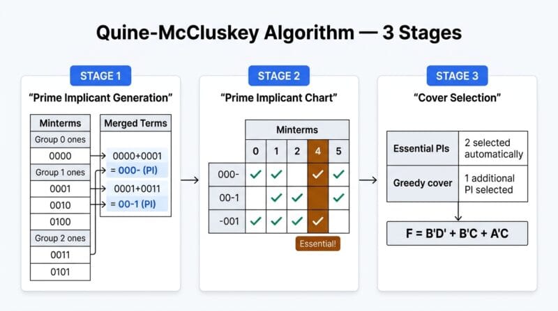
The Quine-McCluskey method is the algorithmic equivalent of the Karnaugh map process — where a K-Map relies on visual grouping that humans perform intuitively, Quine-McCluskey performs the same minimization systematically through combinatorial comparison. The process has three distinct stages. Stage one generates all prime implicants: start with the minterms as one-bit binary strings, group them by number of 1-bits (Hamming weight), then compare adjacent groups looking for pairs that differ in exactly one bit position. When a difference is found, replace that bit with a dash (don’t care) and record the merged term. Repeat until no more merges are possible. Every term that was never merged is a prime implicant — a minimal group of cells that cannot be absorbed into a larger valid group.
Stage two constructs the prime implicant chart: a matrix with minterms as columns and prime implicants as rows, with a mark wherever a prime implicant covers a minterm. Any minterm covered by exactly one prime implicant forces that prime implicant into the solution — these are essential prime implicants. Stage three covers any remaining uncovered minterms using additional prime implicants. The greedy approach selects the prime implicant covering the most uncovered minterms at each step. Petrick’s Method instead builds a Boolean product of sums from the chart and multiplies it out to find all possible complete covers — identifying every set of prime implicants that covers all minterms, then selecting the sets of minimum size. This tool implements both approaches, with Petrick’s capped at 1024 product terms for browser performance on large problems.
🟡 K-Map Grouping Rules — What Makes a Valid Group and Why Size Matters
Karnaugh map cells are arranged so that adjacent cells (horizontally and vertically) differ in exactly one variable — the Gray code ordering (00, 01, 11, 10) rather than binary counting (00, 01, 10, 11) ensures this property. When cells with F=1 are adjacent, they can be grouped and the differing variable cancels out of the product term. A group of 2 adjacent 1-cells eliminates one variable. A group of 4 eliminates two variables. A group of 8 eliminates three. For an n-variable K-Map, a group of 2ᵏ cells produces a term with n−k literals. The largest valid groups produce the fewest literals — maximizing group size is the primary objective of K-Map minimization.
Groups must always be powers of 2 — groups of 3, 5, 6, or 7 are never valid. Groups wrap around edges: the left and right edges of a K-Map are logically adjacent, as are the top and bottom edges. In a 4-variable K-Map, the four corners form a valid group of 4 — each corner is adjacent to the two other corners sharing its row or column through wrap-around. Don’t care cells (X) can be included in any group if they help enlarge it — they cost nothing and can only improve the minimization. Once minimization is complete, don’t cares that were not included in any group take whatever value is more convenient for the implementation (hardware can ignore them). A cell with F=1 may be covered by multiple groups — every 1 must be covered by at least one group, but being covered multiple times is acceptable and sometimes necessary to allow larger groups.
🟢 Petrick’s Method vs Greedy — When the Difference Matters
The greedy algorithm for prime implicant selection is fast and usually produces a minimal or near-minimal result — for most K-Map problems in textbooks and coursework, it gives the same answer as Petrick’s Method. The difference appears in cases where multiple prime implicants cover the same set of remaining minterms with equal cost. A greedy algorithm breaks these ties arbitrarily, which means it may select a valid but non-unique solution without indicating that alternatives exist. Petrick’s Method guarantees finding every minimal cover — all solutions with the same minimum number of product terms and the same total literal count. When a professor asks for “the minimized expression” and there are two equally minimal forms, Petrick’s Method reveals both, which matters for circuit implementation choices where component availability or wiring topology might favor one solution over another.
- 🔵 SOP (Sum of Products) minimizes the 1-cells — the resulting AND-OR two-level circuit directly implements the expression. Each product term maps to an AND gate; the sum maps to an OR gate combining all AND outputs.
- 🟠 POS (Product of Sums) minimizes the 0-cells — the resulting OR-AND two-level circuit is the dual structure. Each sum term maps to an OR gate; the product maps to an AND gate combining all OR outputs. POS is preferred when the number of 0-cells is smaller than the number of 1-cells.
- 🟣 6-variable K-Maps are rarely used by hand because the four-map structure is difficult to visualize — corner adjacencies between maps require tracking which edges of different sub-maps are logically adjacent. The solver handles this automatically through its index mapping, making 6-variable minimization practical in a browser tool where it would be error-prone by hand.
🟡 HDL Output Formats — What Each Language Is Used For
Verilog and VHDL are the two dominant hardware description languages for digital logic design. Verilog, developed at Gateway Design Automation in 1984, uses a C-like syntax with & for AND, | for OR, ~ for NOT, and ^ for XOR. The assign keyword creates a continuous assignment — a combinational logic statement that updates immediately whenever any input changes. SystemVerilog extends Verilog with additional data types and behavioral constructs; the always_comb block is the SystemVerilog-recommended way to describe combinational logic because the simulator automatically infers the sensitivity list rather than requiring manual specification.
VHDL (VHSIC Hardware Description Language), developed under US Department of Defense initiative in the 1980s, uses English-word operators (and, or, not, xor) and requires explicit type declarations — STD_LOGIC for single-bit signals, STD_LOGIC_VECTOR for buses. A VHDL design always consists of at least two parts: the entity declaration (the interface — what signals go in and out) and the architecture body (the implementation). The C and Python outputs are useful for software simulation of logic functions — testing Boolean expressions in unit test frameworks, generating expected outputs for verification testbenches, or embedding logic functions in embedded systems firmware where a hardware implementation is not needed. Use our Digital Logic Studio Pro to generate all five formats from any K-Map solution. For deeper coverage see our complete K-Map and Boolean logic guide.
What is the maximum number of variables this K-Map solver supports?
The solver supports 2 through 6 variables. A 6-variable K-Map contains 64 cells (2⁶) rendered as four 4×4 grids, one for each combination of the first two variables (AB = 00, 01, 11, 10). The Quine-McCluskey algorithm runs on all 64 cells simultaneously regardless of display layout. Petrick’s Method on 6-variable problems with many minterms can generate a large number of product terms during expansion — the implementation caps at 1024 product terms to maintain browser responsiveness. For most practical 6-variable problems with reasonable minterm counts, this limit is not reached.
What does “don’t care” (X) mean in a K-Map and how does it help?
A don’t care (X) represents an input combination that either never occurs in the real system (an invalid state) or whose output value doesn’t matter for correct operation. Since the output can be either 0 or 1 for a don’t care cell, the minimization algorithm assigns it whichever value allows the largest possible groupings. Don’t cares can only reduce the number of product terms in the minimized expression — they never increase it. In sequential logic, unused state encodings are common sources of don’t cares. Click any F cell until it shows X to mark it as a don’t care.
How does the Boolean expression parser handle operator precedence?
The Boolean expression evaluator follows standard operator precedence: NOT (‘) has the highest precedence, AND (implicit concatenation or ·) is second, and OR (+) has the lowest. So AB' + CD evaluates as (A AND (NOT B)) OR (C AND D). Parentheses override precedence as in standard algebra. The evaluator replaces variable names with their binary values for each row of the truth table, then applies the operators. XOR uses the ^ symbol. For complex nested expressions, adding explicit parentheses is recommended to ensure the intended grouping.
What is the difference between canonical SOP and minimized SOP?
Canonical SOP (also called the standard SOP or sum of minterms) represents every minterm as a full product term using all n variables — every variable appears in either complemented or uncomplemented form. For a 4-variable function with minterm 5 (binary 0101), the canonical minterm is A’BC’D. The canonical SOP is unique and maximally expanded. Minimized SOP (what the K-Map produces) groups minterms into prime implicants, eliminating one variable per grouping step. The minimized expression is smaller and directly maps to a two-level AND-OR gate circuit with fewer gates and literals.
Why are NAND and NOR called universal gates?
NAND and NOR are called universal gates because any Boolean function — and therefore any logic circuit — can be implemented using only NAND gates or only NOR gates, without needing any other gate type. This matters because NAND gates are the fundamental building block of CMOS logic (the technology used in virtually all modern digital chips) — they are faster and use less power than equivalent AND-OR combinations. In practice, most synthesis tools automatically convert AND-OR-NOT networks to NAND-NAND or NOR-NOR equivalents during technology mapping for silicon implementation. The Universal Gate Converter in the Gate Simulator tab shows the conversion rules.
Can the Verilog output be used directly in Xilinx Vivado or Intel Quartus?
Yes, with minor additions. The generated Verilog module uses standard synthesizable Verilog syntax compatible with Vivado, Quartus, and other synthesis tools. You may need to add timing constraints (.xdc for Vivado, .sdc for Quartus) and pin assignments separately. The module instantiation line would be logic_minimized uut(.A(A), .B(B), .C(C), .D(D), .F(F)); in a testbench or top-level design. For FPGA synthesis, ensure the output port is connected to a physical pin through your constraint file. The SystemVerilog output is also synthesizable in both tools.
What is the Gray code and why does the K-Map use it?
Gray code is a binary numeral system where adjacent values differ in exactly one bit — the sequence for 2 bits is 00, 01, 11, 10 rather than binary counting 00, 01, 10, 11. The K-Map uses Gray code ordering for its row and column headers because the defining property of a K-Map — adjacent cells differ in one variable — requires that the physical adjacency of cells matches the single-variable-change property. If binary counting were used instead, cells 01 and 10 would be physically adjacent but would differ in two variables simultaneously, which would break the grouping rules. Gray code ensures the visual adjacency exactly corresponds to single-variable difference.
How does the gate simulator handle the case where a gate’s output feeds back into an earlier gate?
The gate chain evaluator processes gates strictly in order from first to last — each gate reads the current output of any preceding gate it references. Feedback loops (where a later gate’s output feeds back into an earlier gate’s input) are not supported because they create sequential logic (flip-flops and latches) rather than combinational logic. The simulator is designed exclusively for combinational circuits where the output depends only on the current inputs with no state or memory. For sequential logic analysis, the K-Map and Boolean tools remain valid for next-state function minimization — you would minimize each output function separately then implement them with feedback externally.
How many prime implicants can the Quine-McCluskey algorithm find for a 6-variable function?
In the worst case, a 6-variable function can have up to several hundred prime implicants. The theoretical maximum grows with the number of variables and the distribution of minterms. For typical engineering problems — functions derived from state machines, decoders, or arithmetic units — the prime implicant count is usually 10–30 for 4-variable problems and 20–80 for 6-variable problems. The solver processes all prime implicants through the chart method and displays the count in the sidebar. The step-by-step trace lists all prime implicant binary strings, which is useful for verifying the algorithm manually against textbook examples.